
t-test
......
t-test ......
What is a t-test
In general terms, a t-test is a statistical procedure for comparing the population mean of some variable between groups. More specifically, the t-test tells us whether the difference in means between groups is statistically significant or whether it could occur by chance.
The t-test is a parametric test and as such makes the following assumptions:
Groups are independent
Groups are normally distributed
Groups have equal within group variance (homoscedasticity)
There are three types of t-test:
One sample t-test
Independent samples t-test
Paired samples t-test
Like many other statistical tests, the t-test can be performed manually. However, this can be very tedious and prone to error. So, for the sake of clarity and brevity, here we will focus on:
Understanding the t-test.
Implementing/performing the t-test in R.
Interpret and draw conclusions from the t-test.
Types of t-test
One Sample t-test
Purpose: Compares the mean of a sample or population with a hypothesized mean, µ.
Method
Independent Samples t-test
Purpose: Compares the means of two completely independent groups/a sample or population with a known population mean, µ.

Paired samples t-test
Purpose: compares the means from the same group at different time points.
Data
Visualization


Example: One-sample t-test
Data
µ=9535
sd=349
Prepare and visualize data

Example: Independent samples t-test


It is believed that 1 litre cartons of a given brand of full cream milk, on average contain 10010mL of milk. We have a random sample of 30 milk carton volume measurements. We wish to determine whether 10010 mL is the true mean volume.
Visualizing the data, the histogram does not demonstrate perfect normality, however it does demonstrate approximate normality perhaps with some right skewness. Again, the boxplot highlights some slight right skewness and the first and last quartiles are not hugely different. Therefore, it is considered reasonable that we assume normality of this dataset for the purpose of conducting a parametric test, i.e. the t-test.
For this example we will set the significance level to 0.05 i.e., α=0.05.


Stating the hypothesis at the start is essential to ensuring correct interpretation. For instance, we should recognize that this is a two-tailed hypothesis test because the alternative hypothesis includes a “not equal to” indicating that if there is a difference it could be in either direction. This is a crucial consideration as it directly determines whether the p-value is one-tailed or two-tailed.
Hypotheses
The p-value (0.9992) is not less than the significance value of 0.05. That is, there insufficient evidence that there is a statistically significant difference between the true mean and the hypothesized vale of 10010. We therefore fail to reject the null hypothesis and conclude that the population mean is volume of milk is 10010 mL.
The p-value, p=2.586e-05 is less than the significance level α=0.05. Therefore, we reject the null hypothesis that there is no statistically significant difference between the means.
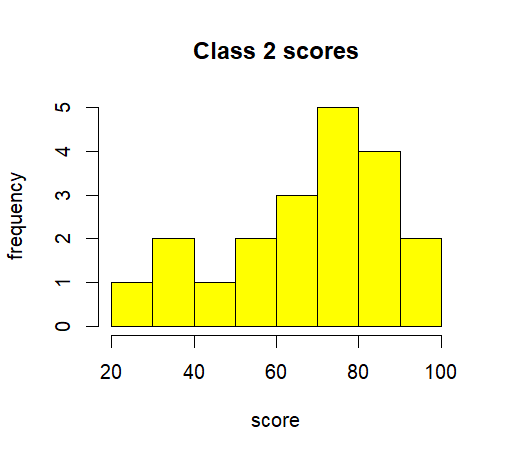
There are two mathematics classes at a particular school, where class1 has regular tutorials and class2 doesn’t. We wish to determine whether class1 performs better, on average, than class2. We will base this on the performance of each class in their upcoming mid-term exam. First we will visualize the data using a histogram and boxplot and we will create a summary of the data.
Hypotheses

Whilst it is clear that the data is not normally distributed, for the purposes of this exercise we will assume approximate normality.
Example: Two-Sample Independent t-test

Conclusion
Considering class2 from the previous example, regular tutorials have now been in place for six months. We wish to determine whether there has been an improvement in class performance in mathematics. This requires a 2 sample paired t-test because we are comparing each student’s result from the first test with their result from the second test, following six months of the tutorial classes being in place.
Data

Visualization

A paired samples t-test assumes that the mean differences are normally distributed. We can test this with a Shapiro-Wilk test of normality.

Define groups
Hypotheses
For the moment we are only interested in establishing whether there is a difference in the means, not the direction (positive/negative) of any difference. Hence we will use the following null and alternative hypotheses.


p=0.2975 so there is insufficient evidence that the means are different. We therefore fail to reject the null hypothesis.


The p-value (1.456e-05) is extremely small and greatly less than 0.05 so we reject the null hypothesis that the data is normally distributed.
This therefore violates the requirement that differences be normally distributed. Strictly speaking, we therefore can’t perform a paired samples t-test to this data.
However, there are possible solutions to this problem:
i) The Central Limit Theorem makes an assumption that a large sample of n>30 can be considered as being normally distributed. For this example we have n=60.
ii) We can use a non-parametric test which does not have the normality requirement e.g., the paired samples Wilcoxon Test
For the purposes of this exercise (example) we will do both tests and compare the results.
Given the allowance of the CLT for large samples, as p<0.05, we reject the null hypothesis that there is no statistically significant difference between the means.

Both the parametric (with the CLT normality assumption) and the non-parametric Paired Samples Wilcoxon yield similar results and we conclude that there is a statistically significant difference between the preScore and postScore means.

Paired samples Wilcoxon Test
Conclusion


Normality of differences
Assign groups and generate summary.

Paired samples t-test
Example: Paired samples t-test